Visualize BAM file alignment at the Leptin gene locus
Our results are in the analysed directory
!ls /home/gea_user/rna-seq-project/kallisto/analyzed
Notice: In this notebook we will be using the Python package genomeview to visualize our BAM alignments. All of our normal shell commands will begin with a ! - python commands will not begin with this character.
lets remind ourselves what each of these directories contain:
| SRA Sample | Sample Name | Folder Name |
|---|---|---|
| SRS1794108 | High-Fat Diet Control 1 | SRR5017135_trimmed.fastq.gz_quant |
| SRS1794110 | High-Fat Diet Control 2 | SRR5017137_trimmed.fastq.gz_quant |
| SRS1794106 | High-Fat Diet Control 3 | SRR5017133_trimmed.fastq.gz_quant |
| SRS1794105 | High-Fat Diet Tumor 1 | SRR5017132_trimmed.fastq.gz_quant |
| SRS1794101 | High-Fat Diet Tumor 2 | SRR5017128_trimmed.fastq.gz_quant |
| SRS1794111 | High-Fat Diet Tumor 3 | SRR5017138_trimmed.fastq.gz_quant |
Optional: We need a copy of the mouse genome to visualize an alignment of these reads. We can use the following command to download the primary assembly from ensembl. This genome has already been provided for you, but you could change the FTP link to download a genome of your choice for a different dataset.
# get mouse genome using wget - uncomment the line below
#!wget ftp://ftp.ensembl.org/pub/release-97/fasta/mus_musculus/dna/Mus_musculus.GRCm38.dna.primary_assembly.fa.gz

# If you import the mouse genome you will also need to decompress it by uncommenting the line below
#!gzip -d Mus_musculus.GRCm38.dna.primary_assembly.fa.gz
We will make a directory for the downloaded genome (mkidr -p) and move (mv) the downloaded genome to the new directory.
!mkdir -p /home/gea_user/rna-seq-project/genomes
!mv /home/gea_user/data/pre-imported/genomes/Mus_musculus.GRCm38.dna.primary_assembly.fa /home/gea_user/rna-seq-project/genomes/
We will now import the genomeview python package
import genomeview
We will specify the datasets (bam) files), as well as the location of our reference genome and the chromosome to visualize (including the start and stop position on the chromosome)
datasets = {"High-Fat Diet Control 1":"/home/gea_user/rna-seq-project/kallisto/analyzed/SRR5017135_trimmed.fastq.gz_quant/pseudoalignments.bam",
            "High-Fat Diet Control 2":"/home/gea_user/rna-seq-project/kallisto/analyzed/SRR5017137_trimmed.fastq.gz_quant/pseudoalignments.bam",
            "High-Fat Diet Control 3":"/home/gea_user/rna-seq-project/kallisto/analyzed/SRR5017133_trimmed.fastq.gz_quant/pseudoalignments.bam",
           "High-fat Diet Tumor 1":"/home/gea_user/rna-seq-project/kallisto/analyzed/SRR5017132_trimmed.fastq.gz_quant/pseudoalignments.bam",
           "High-fat Diet Tumor 2":"/home/gea_user/rna-seq-project/kallisto/analyzed/SRR5017128_trimmed.fastq.gz_quant/pseudoalignments.bam",
           "High-fat Diet Tumor 3":"/home/gea_user/rna-seq-project/kallisto/analyzed/SRR5017138_trimmed.fastq.gz_quant/pseudoalignments.bam"}

reference = "/home/gea_user/rna-seq-project/genomes/Mus_musculus.GRCm38.dna.primary_assembly.fa"
chrom = "chr6"
start = 29060195
end = 29073877
visualization = genomeview.visualize_data(datasets, chrom, start, end, reference)
Finally, we can visualize the three bam files for each of the control/high-fat diets. The blue tick-marks represent individual RNA-Seq reads that map to this region of the genome (the leptin gene). Clearly, in the mouse tumor samples from the high-fat diet mice, expression of this gene is greatly increased. Although each replicated experiment does not have exactly the same number of mapped reads, there is a clear difference. Further statistical analysis would allow us to further describe the signifigance of the difference.
visualization
Visualizing at UCSC Genome Browser
You can also use the URLs above to import your data a track on the UCSC Genome Browser.
- Go to the USCS Genome Browser and select "Mouse"
- Under "Postion/Sear Term" type in "Lep" and choose the first option (Mus musculus leptin (Lep), mRNA. (from RefSeq NM_008493)); then click "Go"

- Under the browser display, click on the "add custom tracks" button.
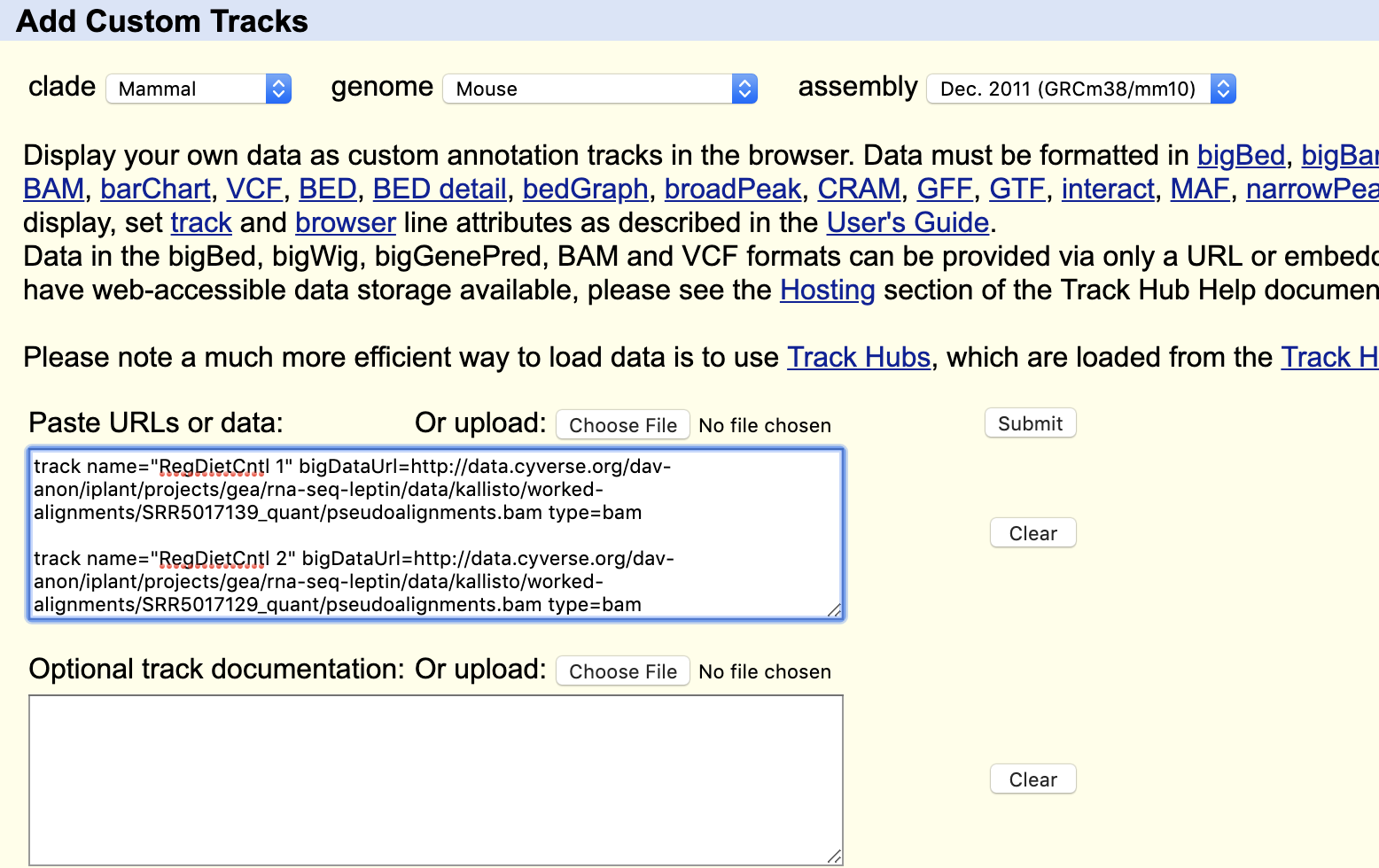
- Copy and paste the formatted URL information from the table below into the "Past URLs or data" box. Do this for all the tracks you wish to view (be sure to copy the entire contents of the tabel cell from "track name" to "type=bam". Put a line of space between each pasted track information.

- Click submit to begin the track upload. On the next screen ("Manage Custom Tracks") click "go" to view in the genome browser.
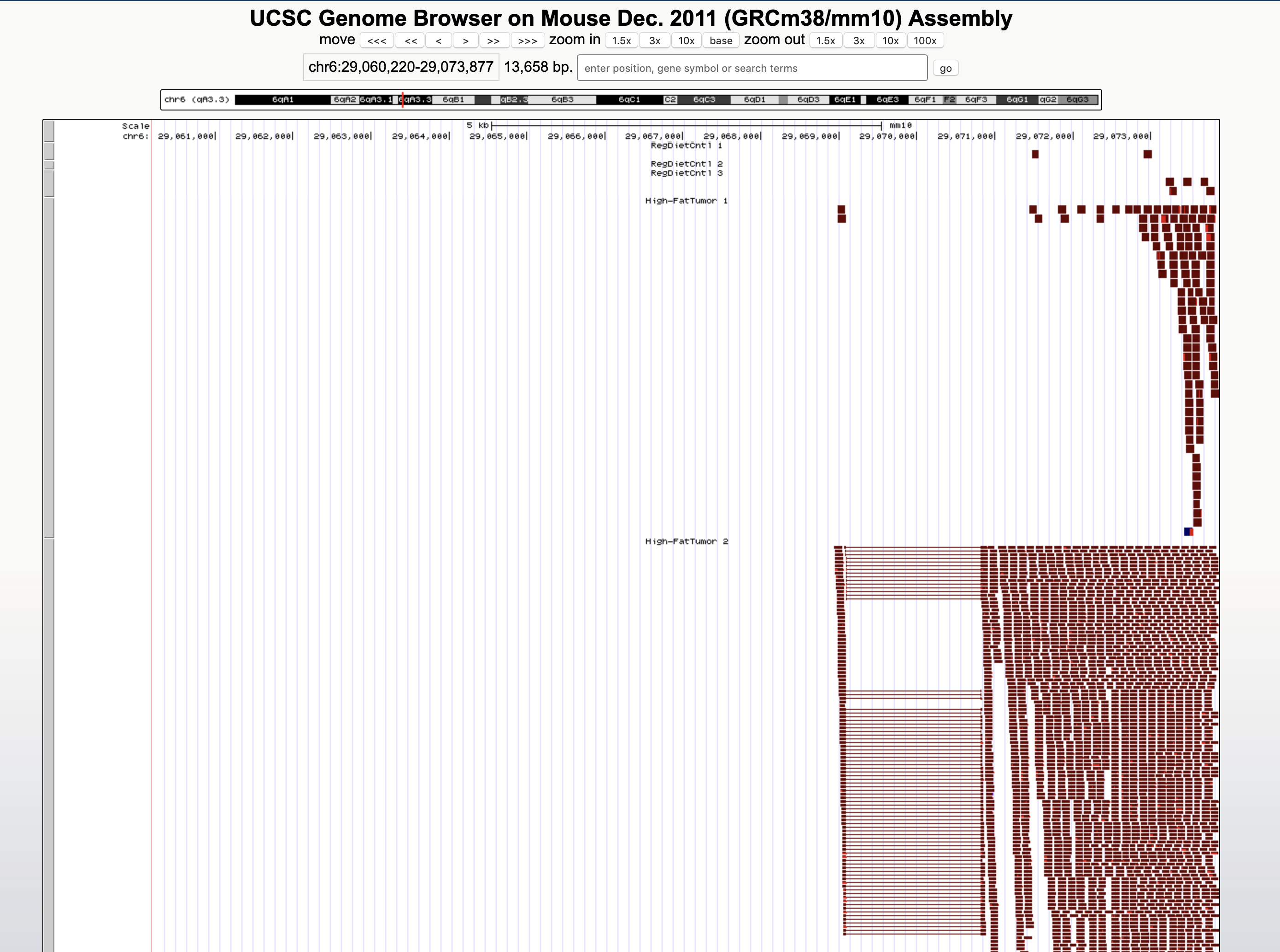
6. You will now have data from your added tracks. For each custom track, you can change the display from "dense" to "squish", "pack", or "full" to see the number of reads (be sure to refresh the display to see the data visualization.

Visualizing in IGV
You can do more extensive visualizations of your data using a genome browser like IGV (Download IGV). After installing IGV you can view the read alignments by performing the following steps:
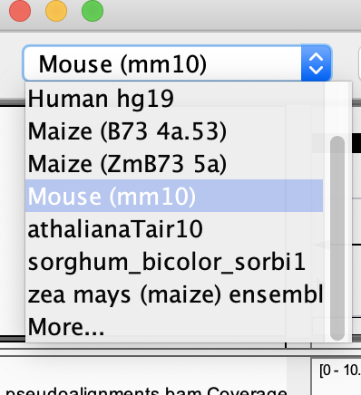
1. In the genome pull-down menu, select the mouse genome: "Mouse (mm10)"

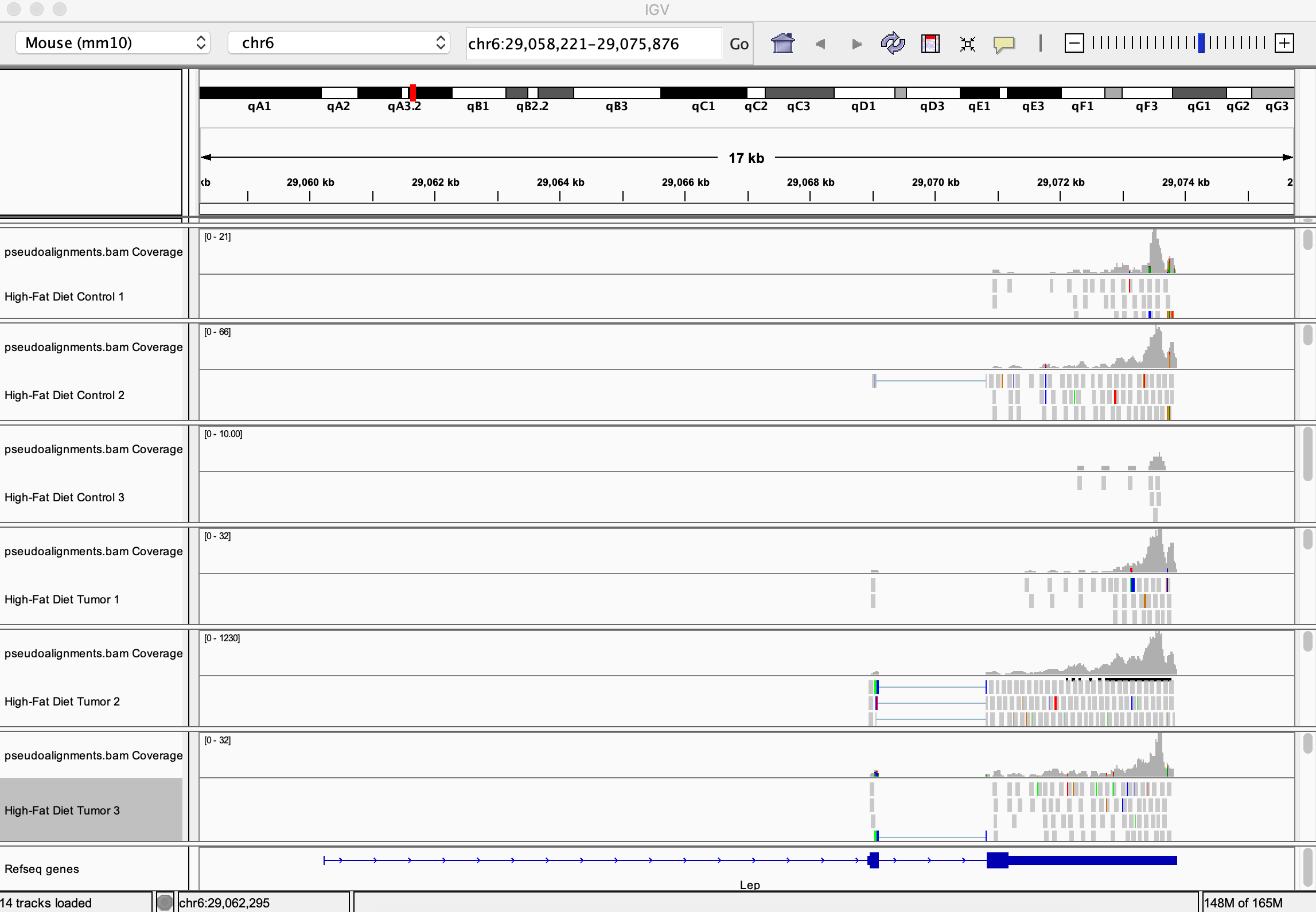
2. In the navigation menu, search for the "Lep" (Leptin) gene and click "Go". The location is:chr6:29,058,221-29,075,876

3. In IGV's "File" menu, select "Load from URL...". In the window that opens, choose a URL from the table below to paste into the "File URL" box. You do not need to provide an Index URL. These URLs correspond to data from the CyVerse Data Store which has already been pre-computed using these notebooks. If you have your own BAM files, you could access the CyVerse Data Store and create a URL to view your file in a genome browser.

4. You can add as many URLs as you wish to view. As you add a track, you may right-click the track name to rename the track. Here is a view of all 6 sets of reads used in this dataset loaded on IGV
